【備忘録】主成分分析と Feature Importance～ Python / Scikit-Learn ～

主成分分析 (Principal Component Analysis, PCA) は、１観測あたり多数の次元／特徴を含む大規模データセットを分析し、最大限の情報量を保持しながらデータの解釈可能性を高め、多次元データの可視化を可能にする手法としてよく利用されています。形式的には、PCA はデータセットの次元を減少させる統計的手法です。これは、データの変動（の大部分）が、初期データよりも少ない次元で記述できるような新しい座標系にデータを線形変換することにより達成できます。

Wikipedia より引用、翻訳・編集

データ解析で頻繁に主成分分析 (PCA) を利用しています。主成分分析をはじめ、よく使用する機械学習の処理部分などは、いつも過去に使ったスクリプトから必要部分をコピペして使い回してしまっているので、思い違いや間違いがあれば、そのままずっと引きずってしまう可能性があります。ちょっと心配になってきたので、簡単なサンプルを使ってスクリプトを整理しようとしています。

今回は Python による主成分分析において、２つのクラスタを特定して、その差に寄与する因子（特徴量）の重要度 (Feature Importance) を評価します。

下記の OS 環境で動作確認をしています。Fedora Linux 38 のデフォルトの Python のバージョンは 3.11.x ですが、一部のライブラリがまだ対応していないので一つ前のバージョン 3.10.y を使っています。

	Fedora Linux 38	x86_64
	Python	3.10.11

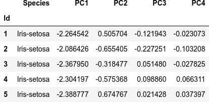
JupyterLab の Notebook 上で動作確認をしています。まず、主成分分析をまとめて処理してしまいます。本ブログ過去記事 [1] で紹介した Iris データセットの主成分分析の処理を、必要な部分だけぎゅっとひとつにまとめました。

import pandas as pd import dataframe_image as dfi from sklearn.pipeline import Pipeline from sklearn.preprocessing import StandardScaler from sklearn.decomposition import PCA   # https://www.kaggle.com/datasets/saurabh00007/iriscsv filename = 'Iris.csv' df = pd.read_csv(filename, index_col=0) cols_x = list(df.columns[0:4]) col_y = df.columns[4] name_target = sorted(list(set(df[col_y])))   # model pipeline for PCA pipe = Pipeline(steps=[     ('scaler', StandardScaler()),     ('PCA', PCA()), ]) features = df[cols_x] pipe.fit(features)   # PCA scores scores = pipe.transform(features) df_pca = pd.DataFrame(     scores,     columns=["PC{}".format(x + 1) for x in range(scores.shape[1])],     index=df.index ) cols_pc = list(df_pca.columns) df_pca.insert(0, col_y, df[col_y].copy()) 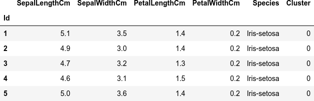dfi.export(df_pca.head(), 'table_061_iris_PCA.png') df_pca.head()

 

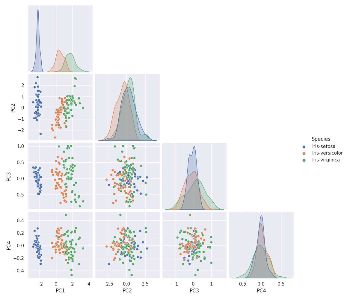
主成分を軸とした散布図を作成します。主成分は４つ（= 説明変数の数）しかないので、全部の組み合わせをプロットします。

import matplotlib.pyplot as plt import seaborn as sns   plt.rcParams['font.size'] = 14   g = sns.pairplot(df_pca, hue=col_y, corner=True) g.fig.suptitle('Iris PCA score scatters', y=1.02)   plt.savefig('iris_061_PCA_scatter.png') plt.show()

 

２つのクラスタの特定

分布の差を調べたい２つのクラスタを特定します。ここでは主成分 PC1 と PC2 に注目し、下記のように赤枠と青丸で囲んだ内側のデータ群を調べることにします。

import matplotlib.patches as patches   fig, ax = plt.subplots() sns.scatterplot(data=df_pca, x='PC1', y='PC2', hue=col_y, ax=ax) ax.set_aspect('equal') ax.legend(loc='center left', bbox_to_anchor=(1, 0.5), fontsize=10) ax.set_title('PC1 vs. PC2')     x1 = -2.5 y1 = -1.0 w1 = 0.5 h1 = 3.0 c1 = patches.Rectangle(xy=(x1, y1) , width=w1, height=h1, fill=False, edgecolor='red') ax.add_patch(c1)   x2 = 1.0 y2 = 0.0 r2 = 0.75 c2 = patches.Circle(xy=(x2, y2), radius=r2, fill=False, edgecolor='blue') ax.add_patch(c2)   plt.savefig('iris_062_PCA_PC1PC2.png') plt.show()

 

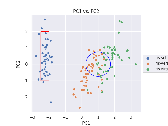
赤枠 (Cluster 0) と青丸 (Cluster 1) で囲んだデータ点に対応する元のデータを、Cluster 列にそれぞれ 0、1 と付けて抽出して連結します。

col_cluster = 'Cluster' # Cluster 0 df_cluster_0 = df[(df_pca['PC1'] > x1) & (df_pca['PC1'] < (x1 + w1)) & (df_pca['PC2'] > y1) & (df_pca['PC2'] < (y1 + h1))].copy() df_cluster_0[col_cluster] = 0 # Cluster 1 df_cluster_1 = df[((df_pca['PC1'] - x2)**2 < r2**2) & ((df_pca['PC2'] - y2)**2 < r2**2)].copy() df_cluster_1[col_cluster] = 1 # concatenate 2 clusters df_cluster = pd.concat([df_cluster_0, df_cluster_1]) dfi.export(df_cluster.head(), 'table_062_iris_PCA_cluster.png') df_cluster

 

Random Forest による分類

特定した２つのクラスタを、ここでは Random Forest の分類器を使って分類します。

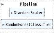
from sklearn.ensemble import RandomForestClassifier from sklearn.preprocessing import StandardScaler   X = df_cluster[cols_x] y = df_cluster[col_cluster]   pipe = Pipeline([     ('scaler', StandardScaler()),     ('RF', RandomForestClassifier(random_state=42)) ]) pipe.fit(X, y)

 

特徴量の重要度の評価

fit した分類結果より、２つのクラスタの差（= 分類）に寄与する因子（特徴量）の重要度 (Feature Importance) を評価します。いくつか算出方法がありますので、主要なやりかたをいくつか利用してみます。

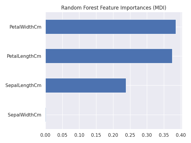
Mean Decrease in Impurity (MDI)

まずは、RandomForest 分類器の feature_importances_ をそのまま利用した場合の計算です。これは、平均不純度変少量（Mean Decrease Impurity; MDI）あるいはジニ重要度（gini importance）と呼ばれる重要度です ^[3]。

feature_names = X.columns   mdi_importances = pd.Series(     pipe['RF'].feature_importances_, index=feature_names ).sort_values(ascending=True) ax = mdi_importances.plot.barh() ax.set_title("Random Forest Feature Importances (MDI)") ax.figure.tight_layout() plt.savefig('iris_071_feature_inportance_mdi.png') plt.show()

 

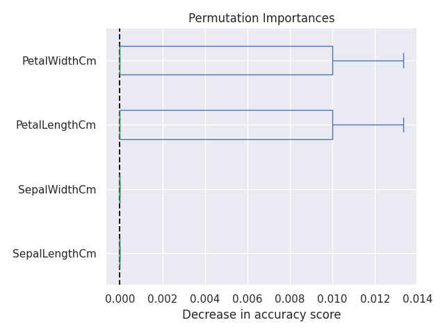
Permutation Importance

Permutation Importance は、元のデータから算出した予測精度と、特徴量の値を並び替えて (permutation) 算出した予測精度を比較して、精度の減少が大きいものをより重要な特徴量と判断しています ^[4]。

from sklearn.inspection import permutation_importance   result = permutation_importance(pipe, X, y, n_repeats=10, random_state=42, n_jobs=2) sorted_importances_idx = result.importances_mean.argsort() importances = pd.DataFrame(     result.importances[sorted_importances_idx].T,     columns=X.columns[sorted_importances_idx], ) ax = importances.plot.box(vert=False, whis=10) ax.set_title('Permutation Importances') ax.axvline(x=0, color='k', linestyle='--') ax.set_xlabel('Decrease in accuracy score') ax.figure.tight_layout() plt.savefig('iris_072_feature_inportance_purmutation.png') plt.show()

 

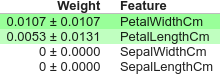
Permutation Importance の算出には、eli5 というパッケージを利用することもできます。

import eli5 from eli5.sklearn import PermutationImportance   perm = PermutationImportance(pipe) perm.fit(X, y) eli5.show_weights(perm, feature_names=X.columns.tolist())

 

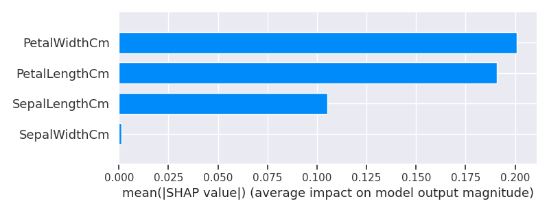
SHAP を用いた特徴量のインパクト

SHAP（SHapley Additive exPlanations）は、協力ゲーム理論のシャープレイ値（Shapley Value）を近似的に算出して機械学習に応用できるようにしたパッケージです。

SHAP では特徴量のインパクトを算出できます、これは各特徴量の貢献度の平均値の絶対値を表示したものです。これによりどの特徴量がモデルに効いているかを確認することができます。これを特徴量の重要度として扱います ^[5]。

import shap shap.initjs()   df_cluster_scaled = pd.DataFrame(pipe['scaler'].fit_transform(X), columns=X.columns)   explainer = shap.TreeExplainer(model=pipe['RF']) shap_values = explainer.shap_values(X=df_cluster_scaled) shap.summary_plot(shap_values[0], df_cluster_scaled, plot_type="bar", show=False) plt.savefig('iris_073_feature_inportance_shap.png') plt.show()

 

確認

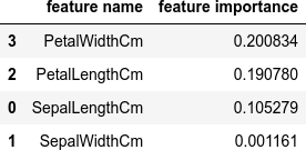
今回は少量のデータをサンプルに使ったためか、特徴量の重要度の算出はどのやり方でも似たような結果になりました。最後の SHAP による特徴量のインパクトから上位２つの特徴量について、クラスタに分類したデータ（標準化済み）を散布図にしました。

import numpy as np   feature_names = X.columns result = pd.DataFrame(shap_values[0], columns=feature_names) vals = np.abs(result.values).mean(0) shap_importance = pd.DataFrame(     list(zip(feature_names, vals)),     columns=['feature name','feature importance'] ) shap_importance.sort_values(     by=['feature importance'],     ascending=False,     inplace=True ) dfi.export(shap_importance, 'table_075_importances_shap.png') shap_importance

 

data_x = shap_importance.iloc[0, 0] data_y = shap_importance.iloc[1, 0]   fig, ax = plt.subplots() sns.scatterplot(data=df_cluster_scaled, x=data_x, y=data_y, hue=list(df_cluster['Species']), ax=ax) ax.set_aspect('equal') ax.legend(loc='center left', bbox_to_anchor=(1, 0.5), fontsize=10) ax.set_title('%s vs. %s' % (data_x, data_y)) ax.set_xlabel('%s (scaled)' % data_x) ax.set_ylabel('%s (scaled)' % data_y) plt.savefig('iris_076_top_2_importances.png') plt.show()

 

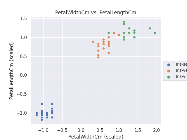
データ数が少なく、特徴量の数も少ないので、わざわざ主成分分析をするまでもない冴えない結果になってしまいました。😅

機械学習というと、予測モデルを作って、その精度が云々という利用が多いのかもしれませんが、自分の場合、多変量解析でこのように分類されたモデルから有意な特徴量を評価するニーズが多いので、備忘録としてまとめました。

トップへ

参考サイト

1. bitWalk's: 【備忘録】主成分分析 ～ Python / Scikit-Learn ～ [2022-12-27]
2. Permutation Importance vs Random Forest Feature Importance (MDI)
3. 決定木アルゴリズムの重要度(importance)を正しく解釈しよう │ キヨシの命題 [2019-09-16]
4. Permutation Importanceを使ってモデルがどの特徴量から学習したかを定量化する | DataRobot [2019-06-13]
5. SHAPを用いて機械学習モデルを説明する l DataRobot [2021-04-14]

 

にほんブログ村


#オープンソース

ChatGPT にコーディングを頼んでみました

ChatGPT ^[1] は、OpenAI が 2022 年 11 月に公開した人工知能チャットボットです。原語の Generative Pre-trained Transformer とは、「生成可能な事前学習済み変換器」という意味になります。OpenAI の GPT-3 ファミリーの言語モデルを基に構築されており、教師あり学習と強化学習の両方の手法で転移学習されています。

Wikipedia より引用

Qiita で ChatGPT に Tkinter で GUI プログラミングをしてもらっている記事 ^[2] を読んで、いやいや、これは凄い！と感動したので、PySide6 ではどうだろうと思って、簡単な GUI プログラムのコーディングを頼んでみました。

ChatGPT とのやりとり

---

PySide6 で Hello World! のGUIプログラムを記述してください。ただし、Hello World!はボタンに表示して、そのボタンをクリックすると Hello World! の文字列を標準出力するようにして下さい。また、GUI 部分は Hello クラスにして再利用できるようにして下さい。

---

以下は、PySide6を使ったHello World!のGUIプログラムです。ボタンをクリックすると、"Hello World!"という文字列が標準出力に出力されます。また、GUI部分は再利用可能なHelloクラスにカプセル化されています。

import sys from PySide6.QtWidgets import QApplication, QMainWindow, QPushButton     class Hello(QMainWindow):     def __init__(self):         super().__init__()           button = QPushButton("Hello World!", self)         button.clicked.connect(self.print_hello)         self.setCentralWidget(button)       def print_hello(self):         print("Hello World!")     if __name__ == '__main__':     app = QApplication(sys.argv)     hello = Hello()     hello.show()     sys.exit(app.exec())

まず、PySide6から必要なクラスをインポートしています。Helloクラスは、QMainWindowを継承しています。init()メソッドでは、QPushButtonを作成し、ウィンドウの中央に配置します。また、clickedシグナルをprint_hello()メソッドに接続します。print_hello()メソッドでは、"Hello World!"という文字列を標準出力に出力します。

最後に、メインウィンドウを作成し、表示するために、QApplicationを作成して、Helloクラスのインスタンスを作成して、show()メソッドを呼び出し、アプリケーションを実行します。

---

イベントループをmain関数にしてもらえますか？

---

はい、イベントループをmain関数に移動して、以下のように書き換えることができます。

import sys from PySide6.QtWidgets import QApplication, QMainWindow, QPushButton     class Hello(QMainWindow):     def __init__(self):         super().__init__()           button = QPushButton("Hello World!", self)         button.clicked.connect(self.print_hello)         self.setCentralWidget(button)       def print_hello(self):         print("Hello World!")     def main():     app = QApplication(sys.argv)     hello = Hello()     hello.show()     sys.exit(app.exec())     if __name__ == '__main__':     main()

ここでは、main()関数が新しく追加され、QApplication、Helloクラスのインスタンスを作成して、show()メソッドを呼び出します。そして、sys.exit()メソッドを呼び出して、アプリケーションが終了するようにします。最後に、if name == 'main':のブロック内で、main()関数を呼び出します。これにより、イベントループがメインスレッドで実行され、アプリケーションが正しく終了されるようになります。

---

流石だね、ありがとう。

---

どういたしまして！何か他に質問があれば、遠慮なく聞いてください。お手伝いできることがあれば、喜んでお手伝いします。

---

実行例

見た目、ちゃんと動きそうなコーディングですが、念の為、実行してみました。

ChatGPT がコーディングした Hello World! の GUI プログラムの実行例

下記の環境で動作確認をしました。

	Fedora Linux 38 beta	(Workstation Edition)	x86_64
	python3-3.11.3-1.fc38.x86_64
	PySide6 6.5.0 (PyPI)

今回は大変簡単なプログラムのコーディングの例でしたが、それでもなかなか感動できる結果でした。果たして痒いところに手が届くような修正がやりとりできるのか興味があるところですが、テーマをしっかり決めてまたやり取りをしてみたいと思います。

トップへ

参考サイト

1. Chat GPT
2. ChatGPT-4 と始める爆速 Python GUI 開発 - Qiita [023-03-18]

 

にほんブログ村


#オープンソース

敢えてスワップファイルを利用する 〜 Fedora Linux 〜

Fedora Linux は Red Hat 社が支援するコミュニティ Fedora Project で開発されているディストリビューションで、最新の技術を積極的に取り込むことで知られています。また Fedora Linux の開発成果が、後にリリースされる Red Hat Enterprise Linux, RHEL に取り込まれています。Fedora Linux は、おおむね春と秋の年二回の頻度で新しい版がリリースされています。

いまどきの Fedora Linux は、デフォルトのインストールではストレージ上にスワップパーティションを作成しません。その代わり、メモリ上に zram という領域が作成されて、ここがスワップ領域に使用されます。参考サイト [1] に詳しい説明があります。

最近の PC はメモリを多く搭載するようになったので、そのメモリ上に圧縮されたスワップ領域を確保しても、普段遣いでは特段の問題は起きません。しかし、一時的に極めて多くの領域を使いたい場合に困ることがあります。

会社で使用しているワークステーション上で、多少時間がかかっても良いから、一時的にメモリの容量を超えるデータを扱いたい事情ができたので、やむなく zram の使用を止め、大きなスワップファイルを用意して対応したので、備忘録にしました。

下記の OS 環境で動作確認をしました。

Fedora Linux 38 beta

(Workstation Edition)

x86_64

zram の使用を停止

参考サイト [2] に従って、zram のサービスを削除してしまいます。

$ sudo dnf remove zram-generator-defaults

btrfs 上にスワップ領域を作成

参考サイト [3] に従って、ファイルシステム btrfs 上にスワップファイルを作成します。

$ sudo btrfs subvolume create /swap $ sudo touch /swap/swapfile $ sudo chattr +C /swap/swapfile $ sudo fallocate --length 95GiB /swap/swapfile $ sudo chmod 600 /swap/swapfile $ sudo mkswap /swap/swapfile

本件では、ワークステーションのメモリ容量が 32GB なのですが、事情により常識外れのサイズ、96GB のスワップファイルを用意しました。

/etc/fstab に下記一行を加えます。

/swap/swapfile none swap swap 0 0

再起動後、スワップファイルがスワップに使われていることを確認します。

$ swapon NAME           TYPE SIZE   USED PRIO /swap/swapfile file  96G 743.5M   -2

SSD 上にスワップ領域を確保することは、寿命の観点で懸念がありますが、ストレージの容量が 2TB あるので、目の前の問題の解決を優先することにして、あまり深く考えないことにします。😅

 

トップへ

参考サイト

1. zram swappingによるRAM節約、高速I/O【Fedora33以降】 - えんでぃの技術ブログ [2021-11-22]
2. Changes/SwapOnZRAM - Fedora Project Wiki
3. Fedora 35 hibernation with swapfile, only for hibernation and resume

 

にほんブログ村


#オープンソース

Fedora Linux 38 (beta) Workstation でサスペンドが起きる！

Fedora Linux は Red Hat 社が支援するコミュニティ Fedora Project で開発されているディストリビューションで、最新の技術を積極的に取り込むことで知られています。また Fedora Linux の開発成果が、後にリリースされる Red Hat Enterprise Linux, RHEL に取り込まれています。Fedora Linux は、おおむね春と秋の年二回の頻度で新しい版がリリースされています。

駄々をこねたわけではないのですが、わがままを認めてもらって、会社のワークステーションには Winodows ではなく Fedora Linux を入れて利用しています。Fedora Linux 38 がベータ版になったので、そろそろアップグレードしてもいいかと思って、先週はじめ、37 からアップグレードしました。

GNOME の設定で自動サスペンドをオフにしても、15 分ぐらいでサスペンドして、リモートデスクトップや httpd などのサービスが止まってしまいます。

GNOME の設定（電源）

そう言えば、半年前に 36 から 37 beta にアップグレードした時もサスペンドが起きて難儀したのを思い出しました。その時もいろいろ調べて回避しようとしていたのですが、やがて勝手にサスペンドしなくなりました。なにか対処をして改善したのかどうか、今となってはあやふやになってしまいました。

今回もいろいろ試してみて、下記参考サイト [1] の方法でうまく回避できたので書き留めておくことにします。

$ sudo systemctl mask sleep.target suspend.target hibernate.target hybrid-sleep.target

なお、他の PC から端末エミュレータでログインして放っておくと、勝手にサスペンドして接続が切れることはなくなりましたが、依然として下記のようなメッセージが出ます。

Fedora Linux にログインしている Tera Term

他にも回避方法があるのかもしれません。ひきつづき調べることにします。まだ、特定の PC にだけ発生する問題なのかも判っていません。

ちなみに、自宅のメイン PC には Fedora Linux Server Edition をインストールしているので、問題が起きていません、というか、そもそも常時稼働させていないので問題にならないだけなのです。

 

トップへ

参考サイト

1. How to Disable Suspend and Hibernation Modes In Linux [2022-12-30]

 

にほんブログ村


#オープンソース