bitWalk's: 2024-05

2024-05-26

CentOS Stream 10 情報 (1)

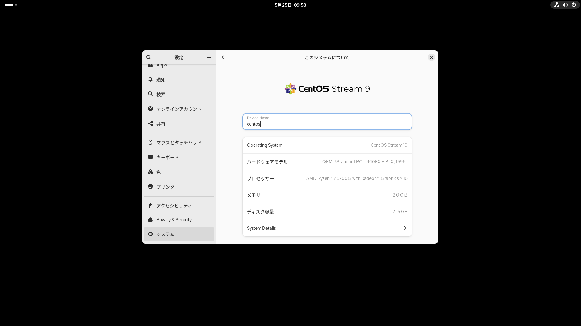
CentOS Stream は、継続的に提供される Red Hat® Enterprise Linux (RHEL) のディストリビューション・アップストリームを、オープンソース・コミュニティのメンバーが Red Hat の開発者と連携して開発、テスト、貢献することができる、Linux® ディストリビューションです。

Red Hat は Red Hat Enterprise Linux ソースコードを CentOS Stream 開発プラットフォームで開発してから、新しい Red Hat Enterprise Linux バージョンをリリースします。Red Hat Enterprise Linux 9 は、CentOS Stream 内で構築された最初のメジャーリリースです。

参考サイト [1] より引用

来年は Red Hat Enterprise Linux 10 がリリースされると予想されますが、その開発版である CentOS Stream の開発が始まっています。まだ正式な CentOS Stream 10 のリリース前ですが、開発版の iso ファイルがダウンロード可能になっています。

毎日のように更新されていますが、ときどき下記から iso ファイルをダウンロードして、仮想環境にインストールして試しています。

CentOS Stream 10（プレリリース版）の入手先

Index of /stream-10/production/latest-CentOS-Stream/compose/BaseOS/x86_64/iso

現時点では GNOME の「このシステムについて」の画面では CentOS Stream 10 のロゴになっておらず CentOS Stream 9 のままです。

CentOS-Stream-10-20240524.0-x86_64-dvd1.iso をインストールしたデスクトップ画面

現時点で、CentOS Stream 10 (CentOS-Stream-10-20240524.0) の構成は以下のようになっています。

Linux kernel: 6.9.0-7
GNOME: 46

カーネルは現時点で Fedora Linux 40 より新しいバージョンですが、RHEL は一旦リリースされるとカーネルのバージョン番号は（10年間）変わらないので、最終的にもっと新しいバージョンになるのかもしれません。

RHEL 10 のリリース・スケジュールは未定ながら、変更内容については明らかになりつつあります。参考サイトにリンクをまとめました。また、なにか変更を確認できれば、本ブログで紹介していく予定です。

トップへ

参考サイト

にほんブログ村

#オープンソース

2024-05-21

【備忘録】HTMLParser の使い方

Python 標準ライブラリの html.parser モジュールで利用できる HTMLParser インスタンスは、HTML データが入力されると、開始タグ、終了タグ、およびその他の要素が見つかる度にハンドラーメソッドを呼び出します。各メソッドの挙動を実装するには HTMLParser サブクラスを使ってそれぞれを上書きして行います。

Python ドキュメント [1] より引用

Web 上の操作を自動化したいとき、PySide6 の QWebEnginePage クラス^[2]のインスタンスに対象 URL を表示して、JavaScript で操作することが多いのですが、単純に特定の情報を抽出したいときは、本体の Python プログラムとのやりとりを面倒に感じています。

Python の標準ライブラリに HTML/XHTML のパーサがあるので使ってみたところ、自分にとっては使い勝手が良かったので、備忘録としてサンプルを掲載しました。

下記の OS 環境で動作確認をしています。

	RHEL 9.4	x86_64
	Python	3.12.1

HTMLParser を使ったサンプルを下記に示しました。このサンプルは、Python ドキュメント [1] に掲載されているサンプルを少し改変したものです。

test_html_parser.py

	from html.parser import HTMLParser


	class MyHTMLParser(HTMLParser):

	def handle_starttag(self, tag, attrs):
	dict_attrs = dict(attrs)
	print("タグのはじめ　 :", tag)
	if len(dict_attrs) > 0:
	print(" └ タグの属性 =", dict_attrs)

	def handle_endtag(self, tag):
	print("タグのおわり　 :", tag)

	def handle_data(self, data):
	print("タグ内の文字列 :", data.strip())


	if __name__ == '__main__':
	parser = MyHTMLParser()
	parser.feed(
	'<html><head><title>テスト（タイトル）</title></head>'
	'<body><h1 id="title">ページタイトル</h1>'
	'<p style="font-family: monospace;">これはテスト用です。</p>'
	'</body></html>'
	)

view raw test_html_parser.py hosted with ❤ by GitHub

３つのメソッド handle_starttag、handle_endtag、handle_data は、継承している HTMLParser クラスのメソッドをオーバーライドしています。

以下が実行例です。

タグのはじめ　 : html
タグのはじめ　 : head
タグのはじめ　 : title
タグ内の文字列 : テスト（タイトル）
タグのおわり　 : title
タグのおわり　 : head
タグのはじめ　 : body
タグのはじめ　 : h1
 └ タグの属性 = {'id': 'title'}
タグ内の文字列 : ページタイトル
タグのおわり　 : h1
タグのはじめ　 : p
 └ タグの属性 = {'style': 'font-family: monospace;'}
タグ内の文字列 : これはテスト用です。
タグのおわり　 : p
タグのおわり　 : body
タグのおわり　 : html

実用的には、抽出したい対象のタグを見つけたらフラグを立てて (handle_starttag)、収集したい文字列を変数に保持して (handle_data)、そのタグが閉じたらフラグを落とす (handle_endtag)、といった処理を加えます。

トップへ

参考サイト

html.parser --- Simple HTML and XHTML parser
QWebEngineView - Qt for Python
Beautiful Soup Documentation
- はじめから BeautifulSoup を利用した方が良かったかもしれません。

にほんブログ村

#オープンソース

2024-05-19

Endless OS 6 を試す

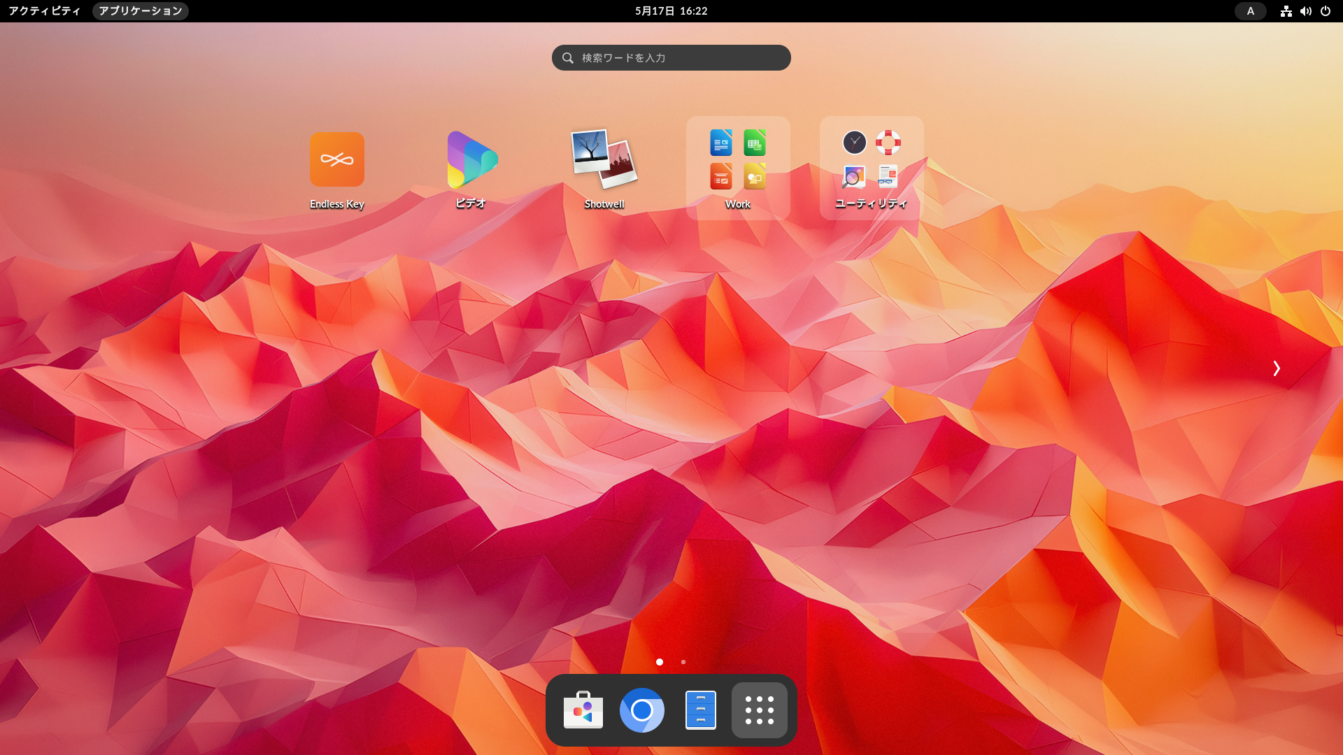
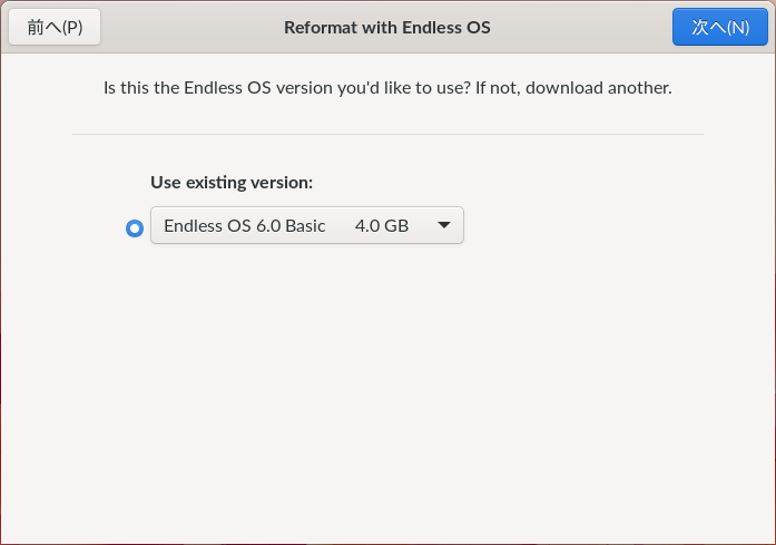
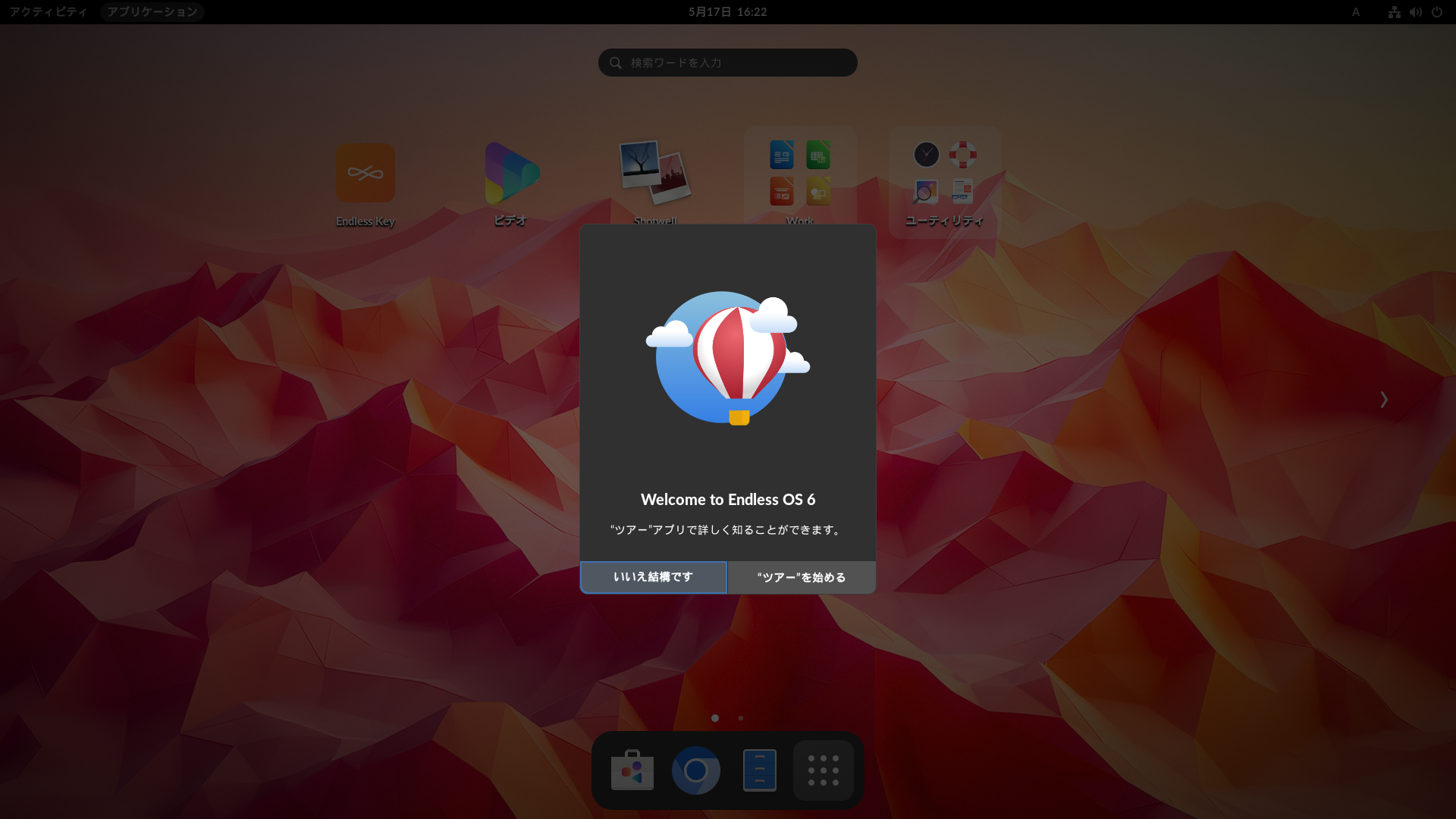
Endless OS 6 が 5 月 14 日にリリースされました^[1]。Endless OS は Debian から派生した Linux ディストリビューションですが、他の多くのディストリビューションと異なり、システムは OSTree で、アプリケーションは Flatpak で管理されています。

Endless OS 6 のデスクトップ画面

Endless OS 財団

2011 年に設立された Endless Mobile, Inc.は、Linux ベースのオペレーティングシステム Endless OS とそのためのリファレンスプラットフォームハードウェアを開発する、米国カリフォルニア州サンフランシスコに本社を置く営利企業でしたが、2020 年 4 月 1 日に非営利団体の Endless OS 財団になりました^[2]。

Endless OS 財団のホームページ [3] によると、Endless OS 財団の使命は、教育へのアクセシビリティを高めることで、世界中の学習者に力を与えることだとされています。そして、デバイス、ユーザーフレンドリーなオペレーティングシステム、豊富な教育リソースなど、学習者に必要不可欠なツールを提供することなどの総合的なアプローチを通じて、この使命を達成するとあります。

Endless OS 財団の活動は以下の３点に要約されます。

Endless OS
- オープンソースのリソース、ツール、アプリがあらかじめ搭載した Endless OS を無償で提供し、すべての人にテクノロジーが手の届きやすいものにします。
Endless Laptop Program
- （パートナー企業が）Endless OS を搭載した手頃な価格のコンピュータとソフトウェアを顧客に提供することで、社会的インパクトを促進します。
Endless Key
- Endless Key は、ChromeOS、Windows、Linux 用の完全無料で安全な（学習用）アプリです。
- コンテンツは、Ted-Ed、Khan Academy、SciGirls などの教育界の世界的リーダーによって提供され、キュレーションされています。
- 学習者は、拡張学習、学問の強化、コーディング、アート＆クラフト、料理、キャリア探索などの興味に基づいたオプションを提供する数十の教育リソースを探索することができます。

Endless OS システム要件

参考サイト [4] のシステム要件をざっくりまとめました。廉価な中華 PC で多く採用されている Realtek の WiFi デバイスが非推奨になっているのが、ちょっと残念です。

CPU: 64bit Intel もしくは AMD プロセッサ (x86_64)
RAM: 最低 2GB、軽量の作業では推奨 4GB、8GB 以上あればマルチタスクにはなお良い。
ストレージ: 最低 32GB
GPU: Intel 内臓 GPU と NVIDIA に対応、AMD 内臓 GPU については対応中。
WiFi: Intel WiFi デバイス推奨、Realtek は非推奨、Linux ドライバがカバーしている Broadcom のデバイスなどには対応。
Webcam: USB 接続の Web カメラには対応。

インストール

ISO イメージのダウンロードサイト

Endless OS Direct Download | Endless OS

今回のリリースがどんなものか確認するため、上記サイトより Endless OS 6.0.0 Basic (eos-eos6.0-amd64-amd64.240514-082534.base.iso) をダウンロードして、仮想マシン (GNOME Boxes) にインストールしました。

ISO ファイルを起動すると最初に言語設定をするダイアログ画面が表示されますので、「日本語」を選択しますが、その後の画面で全面的に日本語のメッセージが表示されるわけではありません。

試用するか、Endless OS をインストールするためにストレージを再フォーマットするか選択する画面になります。右側の Reformat をクリックします。

インストールする Endless OS の確認画面です。右上の 次へ (N) ボタンをクリックして次に進みます。

インストール先のメディアを選択します。ここではそのまま右上の 次へ (N) ボタンをクリックして次に進みます。

なぜか再び言語設定のダイアログ画面（？）が表示されます。ここではそのまま右上の 次へ (N) ボタンをクリックして次に進みます。

インストールがはじまります。

インストールが終わると Power Off ボタンが表示されるので、クリックしてシャットダウンします。

シャットダウン後、インストールメディアを取り出します。

再起動すると GNOME の設定画面が表示されます。日本語の入力メソッドは（従来の Anthy ではなく）Mozc が利用できるようです。右上の 次へ (N) ボタンをクリックして次に進みます。

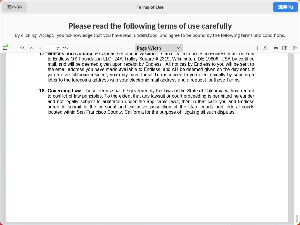
Term of Use（利用規約）が表示されるので、下まで読んで、右上の 適用 (A) ボタンをクリックして次に進みます。

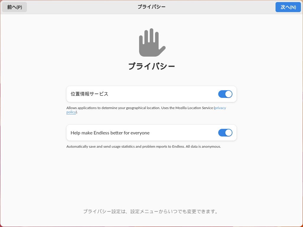
プライバシーを設定して、右上の 次へ (N) ボタンをクリックして次に進みます。

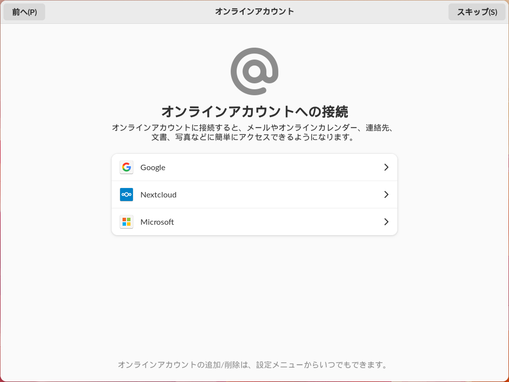
オンラインアカウントへの接続は必要があれば後でもできるので、ここでは右上の スキップ (S) ボタンをクリックして次に進みます。

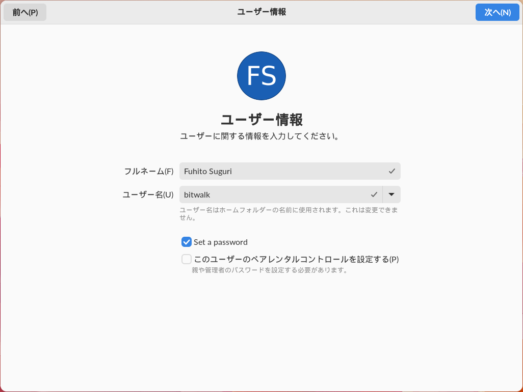
ユーザーアカウントを設定して、ここでは Set a password にチェックを入れて、右上の 次へ (N) ボタンをクリックして次に進みます。

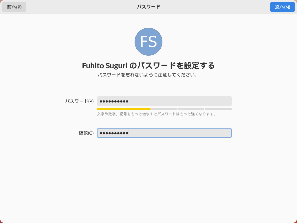
ユーザーアカウントのパスワードを設定して、右上の 次へ (N) ボタンをクリックして次に進みます。

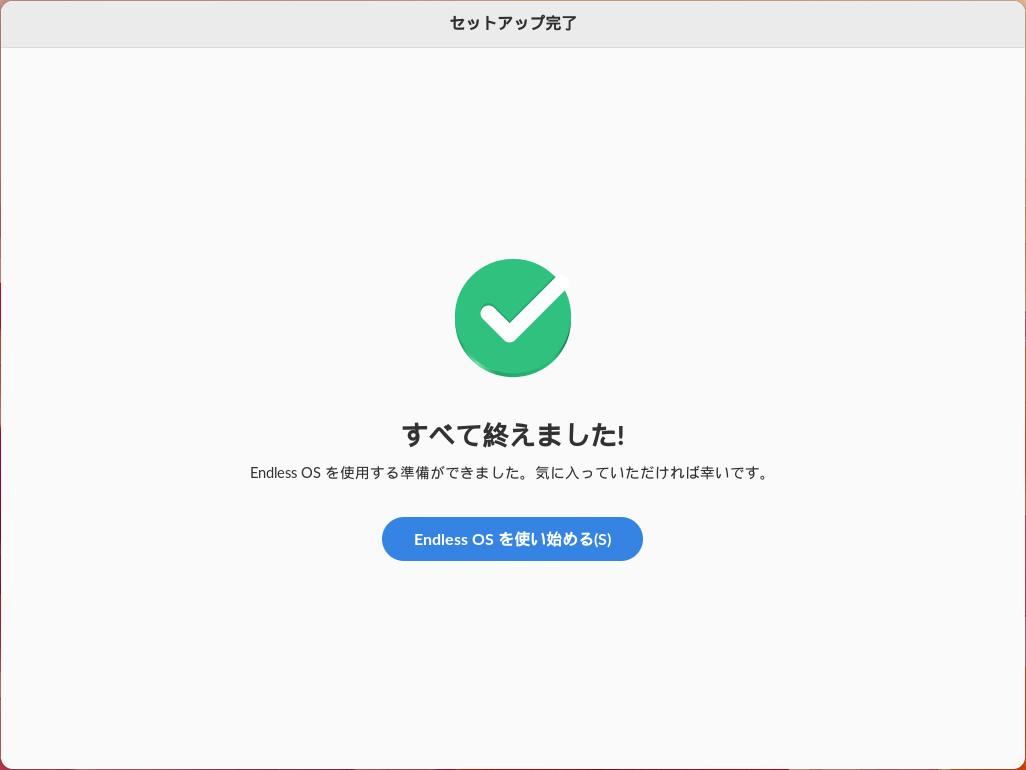
以上で初期設定は終了です。Endless OS を使い始める (S) ボタンをクリックします。

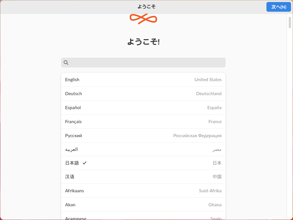
最初にツアーを見るかどうか選択します。

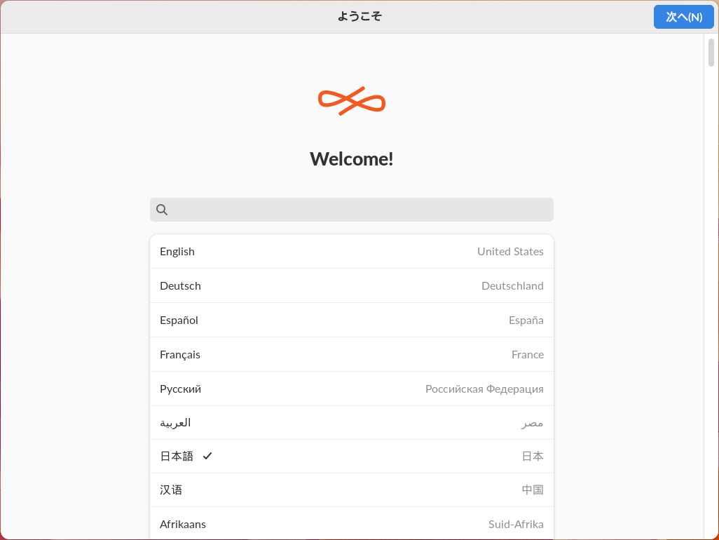
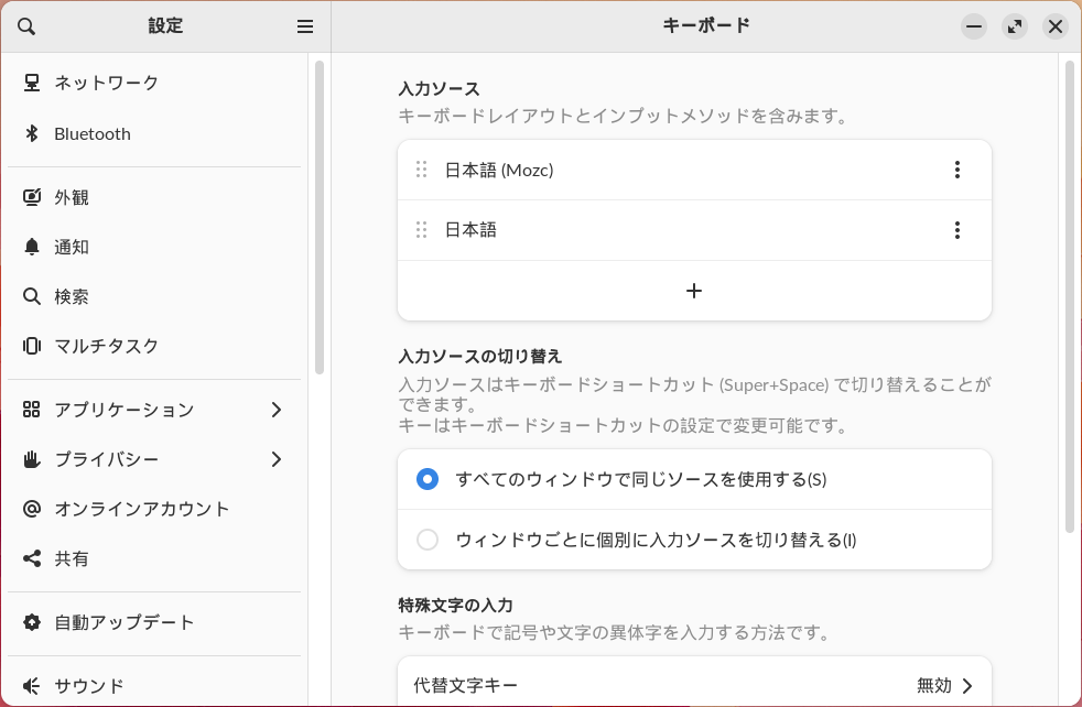
日本語の設定

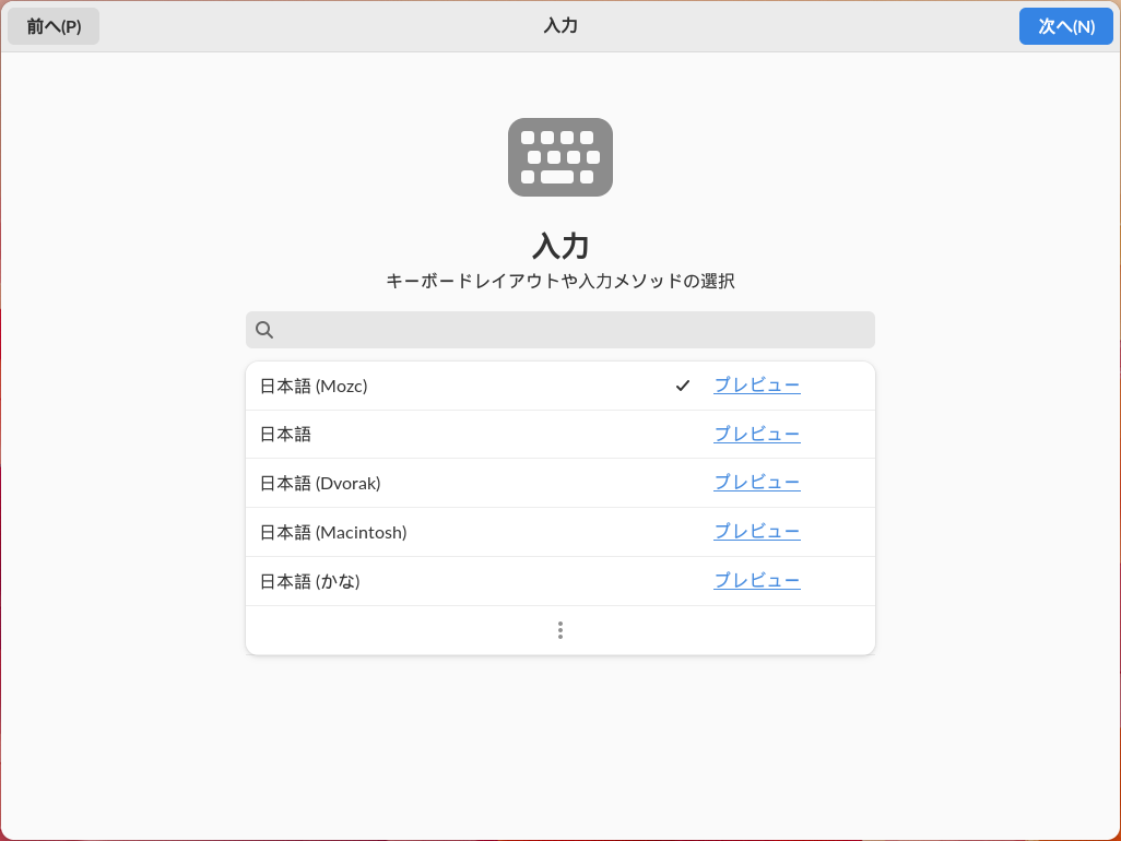
言語設定を二回、入力メソッドを Mozc に設定したのに、すぐに日本語変換ができるわけではなく、キーボードのレイアウトも日本語向けになっていませんでした。結局、GNOME の「設定」で、キーボードに日本語を追加して再起動後、（左 Alt + Space で入力メソッドを切り替えて）漢字変換ができるようになりました。

Endless Key を起動してみたものの…

デスクトップ上に Endless Key のアイコンがあるので、ダブルクリックして起動してみましたが、（当然ながら）英語向けの内容です。紹介できるほど、コンテンツが腹落ちしていないので、少し使ってみてから内容をまとめたいと思います。

Endless Key をはじめて起動

トップへ

参考サイト

Getting Started with Endless OS 6 [2024-05-14]
Launching Endless OS Foundation [2021-01-05]
Endless OS Foundation | Home
Hardware support | Support & Training | Endless OS Foundation

にほんブログ村

#オープンソース

2024-05-16

QLCDNumber と QTimer ～ PySide6

PySide (Qt for Python) は、Qt（キュート）の Python バインディングで、GUI などを構築するためのクロスプラットフォームなライブラリです。Linux/X11, macOS および Microsoft Windows をサポートしています。配布ライセンスは LGPL で公開されています。

GUI アプリで決まった間隔で表示の更新などの処理をさせたい場合、QTimer を利用すると簡単に処理を実装できます。

今回のテーマ

PySide6 の QLCDNumber と QTimer クラスを利用して、シンプルなデジタル時計アプリを作ります。

下記の OS 環境で動作確認をしています。

	RHEL 9.4	x86_64
	Python	3.12.1
	PySide6	6.7.0

メインの PC に Fedora Linux を利用していましたが、今月初めに dnf update でパッケージを更新した後、Fedora Linux 40 上 venv で利用している PySide6 アプリがコアダンプを吐いて利用できなくなりました。原因がわからず、日々利用している自作アプリに支障が出たので、やむなく RHEL に切り替えています^[3]。

サンプルと実行例を以下に示しました。

qt_lcdnumber.py

	import datetime
	import sys

	from PySide6.QtCore import QTimer
	from PySide6.QtWidgets import (
	QApplication,
	QLCDNumber,
	QVBoxLayout,
	QWidget,
	)


	class Example(QWidget):
	def __init__(self):
	super().__init__()
	self.setFixedSize(200, 50)
	self.setWindowTitle('Clock')

	box = QVBoxLayout()
	box.setContentsMargins(0, 0, 0, 0)
	self.setLayout(box)

	self.lcd = QLCDNumber(self)
	self.lcd.setDigitCount(8)
	self.lcd.display('00:00:00')
	box.addWidget(self.lcd)

	timer = QTimer(self)
	timer.timeout.connect(self.update_time)
	timer.start(1000)

	def update_time(self):
	dt_now = datetime.datetime.now()
	self.lcd.display(dt_now.strftime('%H:%M:%S'))


	def main():
	app = QApplication(sys.argv)
	ex = Example()
	ex.show()
	sys.exit(app.exec())


	if __name__ == '__main__':
	main()

view raw qt_lcdnumber.py hosted with ❤ by GitHub

qt_lcdnumber.py の実行例

QTimer クラスを使用するには、QTimer のインスタンスを作成し、timeout() シグナルを適切なスロット（処理するメソッド）に接続し、msec で間隔を指定した start() メソッドを呼び出します。以降、指定された間隔で timeout() シグナルが発せられます。

timer = QTimer(self)
timer.timeout.connect(self.update_time)
timer.start(1000)

本サンプルでは 1000 msec = 1 sec 間隔で timeout() シグナルが発せられるようにして self.update_time() メソッドで QLCDNumber クラスのインスタンスの時刻表示を更新しています。

トップへ

参考サイト

にほんブログ村

#オープンソース

登録: 投稿 (Atom)

bitWalk's

2024-05-26

CentOS Stream 10 情報 (1)

参考サイト

2024-05-21

【備忘録】HTMLParser の使い方

参考サイト

2024-05-19

Endless OS 6 を試す

Endless OS 財団

Endless OS システム要件

インストール

日本語の設定

Endless Key を起動してみたものの…

参考サイト

2024-05-16

QLCDNumber と QTimer ～ PySide6

参考サイト

AddToAny

ブログアーカイブ

ノート

ラベル

Links

ページビューの合計

bitWalk's

2024-05-26

CentOS Stream 10 情報 (1)

参考サイト

2024-05-21

【備忘録】HTMLParser の使い方

参考サイト

2024-05-19

Endless OS 6 を試す

Endless OS 財団

Endless OS システム要件

インストール

日本語の設定

Endless Key を起動してみたものの…

参考サイト

2024-05-16

QLCDNumber と QTimer ～ PySide6

参考サイト

AddToAny

ブログ アーカイブ

ノート

ラベル

Links

ページビューの合計

ブログアーカイブ