PLS 回帰, Partial Least Squares Regression(部分的最小二乗回帰)とは、目的変数 Y を予測するために係数を最適化する手法のひとつです。前回は、R で動作確認した PLS 回帰の使い方を、少し形を変えて Python と Scikit-Learn でも確認しましたが [1]、今回は参考サイト [2] で紹介されている方法で、PLS 回帰における変数選択の重要性について確認しました。
下記の OS 環境で動作確認をしています。

|
Fedora Linux 38 | x86_64 |
| Python | 3.11.3 | |
| JupyterLab | 4.0.2 | |
| scikit-learn | 1.2.2 | |
| matplotlib | 3.7.1 |
本記事は参考サイト [2] に従って、別のサンプルで動作結果をして、それを備忘録にすることが目的なので、統計的解釈に深くは立ち入っていないことをご了承下さい。また、あとで得た知見で書き直したり書き足したりすることもあります。
データセット
前回の PLS の記事 [1] で使ったデータセットの gasoline データを利用しました(下記のサイト)。
具体的には以下のファイルを利用します(本記事で使用するのは gasoline.csv のみです)。
- gasoline.csv
- octane.xlsx
また、上記のリポジトリにあるサンプルプログラム plsr_example.py には、読み込んだファイルを整理してデータセットとして扱いやすいように編集してくれる関数がありましたので、少し修正したものを利用しています。
import numpy as np
import pandas as pd

def import_dataset(ds_name='octane'):
    """
    ds_name: Name of the dataset ('octane', 'gasoline')
    Returns:
    wls: Numpy ndarray: List of wavelength
    xdata: Pandas DataFrame: Measurements
    ydata: Pandas Series: Octane numbers
    """

    if ds_name == 'octane':
        oct_df = pd.read_excel('octane.xlsx')
        wls = np.array([int(i) for i in oct_df.columns.values[2:]])
        xdata = oct_df.loc[:, '1100':]
        ydata = oct_df['Octane number']
    elif ds_name == 'gasoline':
        import re

        gas_df = pd.read_csv('gasoline.csv')
        reg = re.compile('([0-9]+)')
        wls = np.array([int(reg.findall(i)[0]) for i in gas_df.columns.values[1:]])
        xdata = gas_df.loc[:, 'NIR.900 nm':]
        ydata = gas_df['octane']
    else:
        exit('Invalid Dataset')

    return wls, xdata, ydata
利用できるデータセットは二種類ありますが、ここでは gasoline を指定してデータを取得します。
dataset = 'gasoline'
#dataset = 'octane'
wls, xdata, ydata = import_dataset(dataset)
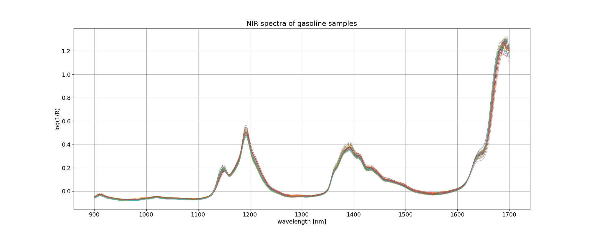
イメージしやすいように、読み込んだ gasoline データについて、波長を横軸にとってプロットしました。凡例を付けませんでしたが、線の色はオクタン価の違いを表しています。
import matplotlib.pyplot as plt
plt.rcParams['font.size'] = 14

fig, ax = plt.subplots(figsize=(20, 8))
ax.plot(wls, xdata.values.T, linewidth=0.5)
ax.set_title('NIR spectra of %s samples' % dataset)
ax.set_xlabel('wavelength [nm]')
ax.set_ylabel('log(1/R)')

plt.grid()
plt.savefig('octane_101.png')
plt.show()
最適モデルの探索 2
このデータ解析の目的は、
octane = f(NIR) = f(NIRwavelength1, NIRwavelength2, ...)
という関数関係を求めて、スペクトルからオクタン価を予測することなのですが、401 個の変数(NIR スペクトル、波長)、60 組のデータでは、従来の重回帰分析を使おうとしても自由度が全然足りなくて解析できません。しかし、401 個のデータは互いに独立した関係にはありません。そこで PLS 回帰を用いて、これら NIR スペクトルから互いに無相関な新しい説明変数(潜在変数)を抽出して、重要度(標準回帰係数)の高い潜在変数から順番に適用して関数関係を求めます。
octane = g(compwavelength1, compwavelength2, ...)
前回 [1] は、成分数を変えて PLS 回帰を実行して、予実の MSE(平均二乗誤差)が最小になる成分数を見つけるというアプローチでした。
今回は 成分数の探索に加えて、401 個の変数(NIR スペクトル、波長)から、オクタン価の予測に寄与する(= MSE を最小にする)変数の組み合わせを選択するというアプローチを取ります。評価基準はクロスバリデーションをした上で MSE が最初になる変数の組み合わせを選ぶことになります。
まず、データをトレーニング用とテスト用の二つに分けます。分ける比率は前回 [1] と揃えました。
from sklearn.model_selection import train_test_split

X_train, X_test, y_train, y_test = train_test_split(xdata, ydata, test_size=0.16, shuffle=False)
X_train, y_train のデータセットを使って、前回と同じように MSE が最小となるように PLS 回帰の成分数を変動させます。そのループの中で、さらに寄与度の低い変数(NIR スペクトル、波長)から一つずつ抜いて PLS 回帰を実行、クロスバリデーションをして MSE を評価します。
なお、計算時間を少しでも減らしたかったので、とりあえず PLS 回帰の最大の成分数を、元の変数の数の1割としました。最適な成分数がこの最大値と同じになるような場合は、この最大値を増やします。
from sys import stdout
import warnings

from sklearn.cross_decomposition import PLSRegression
from sklearn.model_selection import cross_val_predict
from sklearn.metrics import mean_squared_error

warnings.simplefilter("ignore")

X = X_train.values
y = y_train
max_comp = int(X.shape[1] / 10)

# Define MSE array to be populated
mse = np.zeros((max_comp, X.shape[1]))

# Loop over the number of PLS components
for i in range(max_comp):

    # Regression with specified number of components, using full spectrum
    pls1 = PLSRegression(n_components=i + 1)
    pls1.fit(X, y)

    # Indices of sort spectra according to ascending absolute value of PLS coefficients
    # sorted_ind = np.argsort(np.abs(pls1.coef_[:, 0]))
    sorted_ind = np.argsort(np.abs(pls1.coef_[0]))

    # Sort spectra accordingly
    Xc = X[:, sorted_ind]

    # Discard one wavelength at a time of the sorted spectra,
    # regress, and calculate the MSE cross-validation
    for j in range(Xc.shape[1] - (i + 1)):

        pls2 = PLSRegression(n_components=i + 1)
        pls2.fit(Xc[:, j:], y)

        y_cv = cross_val_predict(pls2, Xc[:, j:], y, cv=5)

        mse[i, j] = mean_squared_error(y, y_cv)

    comp = 100 * (i + 1) / (max_comp)
    stdout.write('\r%d%% completed' % comp)
    stdout.flush()

stdout.write('\n')

# Calculate and print the position of minimum in MSE
mseminx, mseminy = np.where(mse==np.min(mse[np.nonzero(mse)]))

print('Optimised number of PLS components:', mseminx[0] + 1)
print('Wavelengths to be discarded', mseminy[0])
print('Optimised MSEP', mse[mseminx, mseminy][0])
stdout.write('\n')
100% completed
Optimised number of PLS components: 27
Wavelengths to be discarded 300
Optimised MSEP 0.02052183734296931
計算の結果、PLS 回帰の最適な成分数は 27、破棄される波長数は 300 となりました。
この最適な PLS モデルでトレーニングデータを予測(クロスバリデーションと比較)した値と測定値とを単回帰したプロットを示しました。
from sklearn.metrics import r2_score

X = X_train.values
y = y_train

# Calculate PLS with optimal components and export values
pls = PLSRegression(n_components=mseminx[0] + 1)
pls.fit(X, y)

# sorted_ind = np.argsort(np.abs(pls.coef_[:, 0]))
sorted_ind = np.argsort(np.abs(pls.coef_[0]))

Xc = X[:, sorted_ind]
opt_Xc = Xc[:, mseminy[0]:]

n_comp = mseminx[0] + 1
wav = mseminy[0]

pls = PLSRegression(n_components=n_comp)

pls.fit(opt_Xc, y)
y_c = pls.predict(opt_Xc)

# Cross-validation
y_cv = cross_val_predict(pls, opt_Xc, y, cv=10)

# Calculate scores for calibration and cross-validation
score_c = r2_score(y, y_c)
score_cv = r2_score(y, y_cv)

# Calculate mean square error for calibration and cross validation
mse_c = mean_squared_error(y, y_c)
mse_cv = mean_squared_error(y, y_cv)

print('R2 calib: %5.3f'  % score_c)
print('R2 CV: %5.3f'  % score_cv)
print('MSE calib: %5.3f' % mse_c)
print('MSE CV: %5.3f' % mse_cv)

# Plot regression
z = np.polyfit(y, y_cv, 1)

fig, ax = plt.subplots(figsize=(8, 8))
ax.scatter(y_cv, y, c='red', edgecolors='k')
ax.plot(z[1] + z[0] * y, y, c='blue', linewidth=1)
ax.plot(y, y, color='green', linewidth=1)
ax.axis('equal')
plt.title('Train data $R^{2}$ (CV): %5.3f' % score_cv)
plt.xlabel('Predicted')
plt.ylabel('Measured')
plt.grid()

plt.savefig('octane_111.png')
plt.show()
R2 calib: 1.000
R2 CV: 0.993
MSE calib: 0.000
MSE CV: 0.016
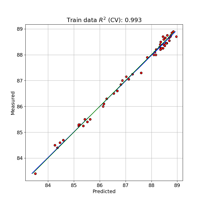
クロスバリデーションをした予測で決定係数が 0.993 となっており、前回よりさらによくフィッティングできています。クロスバリデーションをしない MSE calib が 0.000( R2 =1.000)になっているのは、ちょっとできすぎの感があります。
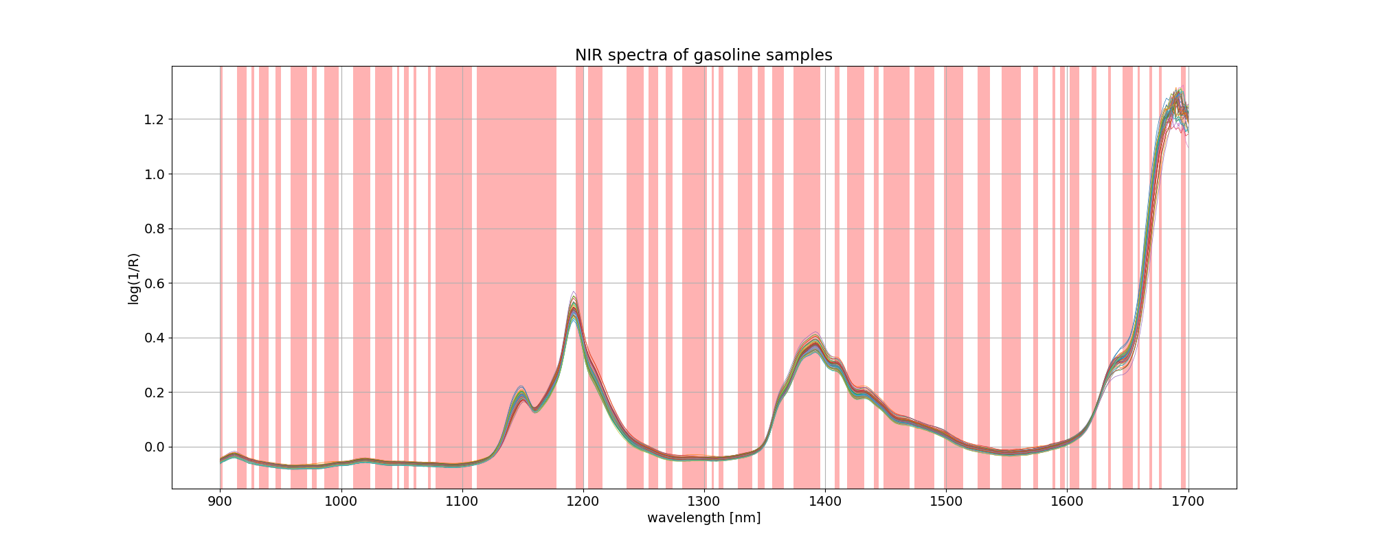
変数選択の結果、使用しなかった(discarded: 破棄した)波長に色を付けると以下のようになります。
# Get a boolean array according to the indices that are being discarded
ix = np.in1d(wls.ravel(), wls[sorted_ind][:wav])

import matplotlib.collections as collections

# Plot spectra with superimpose selected bands
fig, ax = plt.subplots(figsize=(20, 8))
ax.plot(wls, xdata.values.T, linewidth=0.5)
ax.set_title('NIR spectra of %s samples' % dataset)
ax.set_xlabel('wavelength [nm]')
ax.set_ylabel('log(1/R)')

collection = collections.BrokenBarHCollection.span_where(
    wls,
    ymin=-1,
    ymax=max(xdata.T),
    where=ix==True,
    facecolor='red',
    alpha=0.3
)
ax.add_collection(collection)
plt.grid()

plt.savefig('octane_112.png')
plt.show()
テストデータで予測
テストデータで PLS のモデルで予測した値と測定値とを単回帰したプロットを示しました。
X = X_test.values
y = y_test

X_test_2 = X[:, sorted_ind]
opt_X_test = X_test_2[:, mseminy[0]:]

# pls.fit(opt_X_test, y)
y_pred = pls.predict(opt_X_test)

# Calculate scores for calibration
score_pred = r2_score(y, y_pred)

# Calculate mean square error for calibration
mse_pred = mean_squared_error(y, y_pred)

print('R2 pred: %5.3f'  % score_pred)
print('MSE pred: %5.3f' % mse_pred)

# Plot regression
z = np.polyfit(y, y_pred, 1)

fig, ax = plt.subplots(figsize=(8, 8))
ax.scatter(y_pred, y, c='red', edgecolors='k')
ax.plot(z[1] + z[0] * y, y, c='blue', linewidth=1)
ax.plot(y, y, color='green', linewidth=1)
ax.axis('equal')
plt.title('Test data $R^{2}$ (Prediction): %.3f' % score_pred)
plt.xlabel('Predicted')
plt.ylabel('Measured')
plt.grid()

plt.savefig('octane_113.png')
plt.show()
R2 pred: 0.808
MSE pred: 0.439
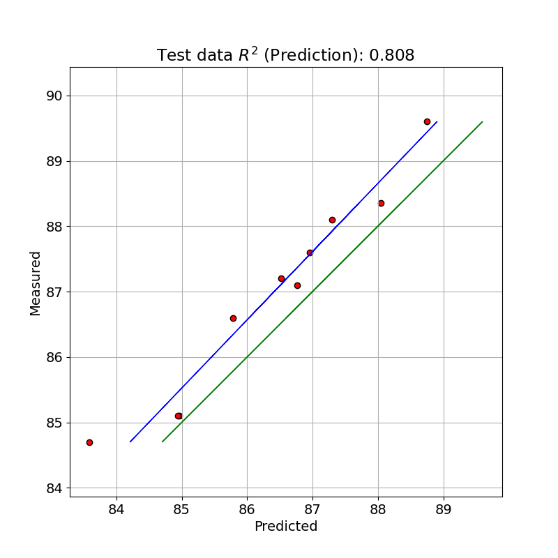
テストデータでは、今回はあまり良いパフォーマンスを得られませんでした。
※ テストデータの評価に間違いがありましたので修正しました。[2023-07-07]
参考サイト
- bitWalk's: 【備忘録】Python/Scikit-learn の PLS を使う [2023-05-27]
- A variable selection method for PLS in Python [2018-07-04]
にほんブログ村

#オープンソース