PLS 回帰, Partial Least Squares Regression(部分的最小二乗回帰)とは、目的変数 Y を予測するために係数を最適化する手法のひとつです。以前、R の pls パッケージを使い方をまとめましたので [1]、python / scikit-learn でも同じように PLS を扱ってみます。
下記の OS 環境で動作確認をしています。

|
Fedora Linux 38 | x86_64 |
| Python | 3.11.3 | |
| JupyterLab | 4.0.0 | |
| scikit-learn | 1.2.2 | |
| matplotlib | 3.7.1 |
ここでは、サイト [2] で紹介されている方法を別のデータセットで確認しています。本記事はその動作結果を備忘録にすることが目的なので、統計的解釈に深くは立ち入っていないことをご了承下さい。また、あとで得た知見で書き直したり書き足したりすることもあります。
データセット
以前 R の pls パッケージの使い方の紹介 [1] で使ったデータセットと同じ gasoline データは、下記のサイトで公開されていましたので、利用させていただきました。
具体的には以下のファイルを利用します(本記事で使用するのは gasoline.csv のみです)。
- gasoline.csv
- octane.xlsx
また、上記のリポジトリにあるサンプルプログラム plsr_example.py には、読み込んだファイルを整理してデータセットとして扱いやすいように編集してくれる関数がありましたので、少し修正して利用しています。
import numpy as np
import pandas as pd

def import_dataset(ds_name='octane'):
    """
    ds_name: Name of the dataset ('octane', 'gasoline')
    Returns:
    wls: Numpy ndarray: List of wavelength
    xdata: Pandas DataFrame: Measurements
    ydata: Pandas Series: Octane numbers
    """

    if ds_name == 'octane':
        oct_df = pd.read_excel('octane.xlsx')
        wls = np.array([int(i) for i in oct_df.columns.values[2:]])
        xdata = oct_df.loc[:, '1100':]
        ydata = oct_df['Octane number']
    elif ds_name == 'gasoline':
        import re

        gas_df = pd.read_csv('gasoline.csv')
        reg = re.compile('([0-9]+)')
        wls = np.array([int(reg.findall(i)[0]) for i in gas_df.columns.values[1:]])
        xdata = gas_df.loc[:, 'NIR.900 nm':]
        ydata = gas_df['octane']
    else:
        exit('Invalid Dataset')

    return wls, xdata, ydata
利用できるデータセットは二種類ありますが、ここでは gasoline を指定してデータを取得します。
dataset = 'gasoline'
#dataset = 'octane'
wls, xdata, ydata = import_dataset(dataset)
取得した wls, xdata, ydata それぞれの内容を確認します。
まず、波長 (wls) です。
print(len(wls))
wls
401
array([ 900,  902,  904,  906,  908,  910,  912,  914,  916,  918,  920,
        922,  924,  926,  928,  930,  932,  934,  936,  938,  940,  942,
        944,  946,  948,  950,  952,  954,  956,  958,  960,  962,  964,
        966,  968,  970,  972,  974,  976,  978,  980,  982,  984,  986,
        988,  990,  992,  994,  996,  998, 1000, 1002, 1004, 1006, 1008,
       1010, 1012, 1014, 1016, 1018, 1020, 1022, 1024, 1026, 1028, 1030,
       1032, 1034, 1036, 1038, 1040, 1042, 1044, 1046, 1048, 1050, 1052,
       1054, 1056, 1058, 1060, 1062, 1064, 1066, 1068, 1070, 1072, 1074,
       1076, 1078, 1080, 1082, 1084, 1086, 1088, 1090, 1092, 1094, 1096,
       1098, 1100, 1102, 1104, 1106, 1108, 1110, 1112, 1114, 1116, 1118,
       1120, 1122, 1124, 1126, 1128, 1130, 1132, 1134, 1136, 1138, 1140,
       1142, 1144, 1146, 1148, 1150, 1152, 1154, 1156, 1158, 1160, 1162,
       1164, 1166, 1168, 1170, 1172, 1174, 1176, 1178, 1180, 1182, 1184,
       1186, 1188, 1190, 1192, 1194, 1196, 1198, 1200, 1202, 1204, 1206,
       1208, 1210, 1212, 1214, 1216, 1218, 1220, 1222, 1224, 1226, 1228,
       1230, 1232, 1234, 1236, 1238, 1240, 1242, 1244, 1246, 1248, 1250,
       1252, 1254, 1256, 1258, 1260, 1262, 1264, 1266, 1268, 1270, 1272,
       1274, 1276, 1278, 1280, 1282, 1284, 1286, 1288, 1290, 1292, 1294,
       1296, 1298, 1300, 1302, 1304, 1306, 1308, 1310, 1312, 1314, 1316,
       1318, 1320, 1322, 1324, 1326, 1328, 1330, 1332, 1334, 1336, 1338,
       1340, 1342, 1344, 1346, 1348, 1350, 1352, 1354, 1356, 1358, 1360,
       1362, 1364, 1366, 1368, 1370, 1372, 1374, 1376, 1378, 1380, 1382,
       1384, 1386, 1388, 1390, 1392, 1394, 1396, 1398, 1400, 1402, 1404,
       1406, 1408, 1410, 1412, 1414, 1416, 1418, 1420, 1422, 1424, 1426,
       1428, 1430, 1432, 1434, 1436, 1438, 1440, 1442, 1444, 1446, 1448,
       1450, 1452, 1454, 1456, 1458, 1460, 1462, 1464, 1466, 1468, 1470,
       1472, 1474, 1476, 1478, 1480, 1482, 1484, 1486, 1488, 1490, 1492,
       1494, 1496, 1498, 1500, 1502, 1504, 1506, 1508, 1510, 1512, 1514,
       1516, 1518, 1520, 1522, 1524, 1526, 1528, 1530, 1532, 1534, 1536,
       1538, 1540, 1542, 1544, 1546, 1548, 1550, 1552, 1554, 1556, 1558,
       1560, 1562, 1564, 1566, 1568, 1570, 1572, 1574, 1576, 1578, 1580,
       1582, 1584, 1586, 1588, 1590, 1592, 1594, 1596, 1598, 1600, 1602,
       1604, 1606, 1608, 1610, 1612, 1614, 1616, 1618, 1620, 1622, 1624,
       1626, 1628, 1630, 1632, 1634, 1636, 1638, 1640, 1642, 1644, 1646,
       1648, 1650, 1652, 1654, 1656, 1658, 1660, 1662, 1664, 1666, 1668,
       1670, 1672, 1674, 1676, 1678, 1680, 1682, 1684, 1686, 1688, 1690,
       1692, 1694, 1696, 1698, 1700])
つぎは、NIR スペクトルのデータ (xdata) です。
import dataframe_image as dfi

print(xdata.shape)
dfi.export(xdata, 'octane_table_001.png', max_cols=10, max_rows=10,)
xdata
(60, 401)
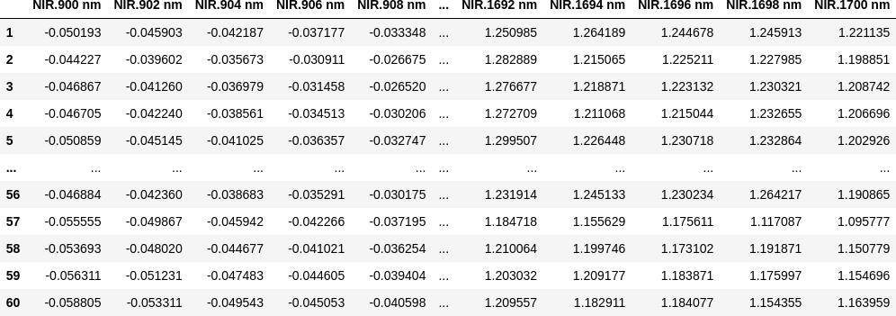
60 rows × 401 columns
そして、対応するオクタン価のデータ (ydata) です。
print(ydata.shape)
ydata.head()
(60,)
1    85.30
2    85.25
3    88.45
4    83.40
5    87.90
Name: octane, dtype: float64
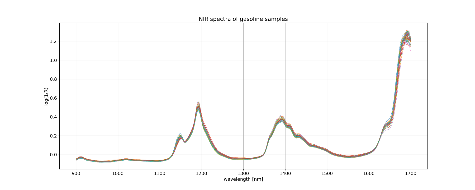
イメージしやすいように、gasoline データについて、波長を横軸にとってプロットしてみました。凡例を付けませんでしたが、線の色はオクタン価の違いを表しています。
import matplotlib.pyplot as plt
plt.rcParams['font.size'] = 14

fig, ax = plt.subplots(figsize=(20, 8))
ax.plot(wls, xdata.values.T, linewidth=0.5)
ax.set_title('NIR spectra of %s samples' % dataset)
ax.set_xlabel('wavelength [nm]')
ax.set_ylabel('log(1/R)')

plt.grid()
plt.savefig('octane_001.png')
plt.show()
最適モデルの探索
このデータ解析の目的は、
octane = f(NIR) = f(NIRwavelength1, NIRwavelength2, ...)
という関数関係を求めて、スペクトルからオクタン価を予測することなのですが、401 個の変数(NIR スペクトル)、60 組のデータでは、従来の重回帰分析を使おうとしても自由度が全然足りなくて解析できません。しかし、401 個のデータは互いに独立した関係にはありません。そこで PLS 回帰を用いて、これら NIR スペクトルから互いに無相関な新しい説明変数(潜在変数)を抽出して、重要度(標準回帰係数)の高い潜在変数から順番に適用して関数関係を求めます。
octane = g(compwavelength1, compwavelength2, ...)
まず、データをトレーニング用とテスト用の二つに分けます。分ける比率は、以前 R の pls パッケージの使い方を紹介 [1] した時と同じにしました。
from sklearn.model_selection import train_test_split

X_train, X_test, y_train, y_test = train_test_split(xdata, ydata, test_size=0.16, shuffle=False)
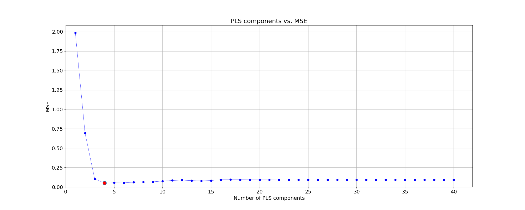
X_train, y_train のデータセットを使って、成分 (component) の数を変えて PLS 回帰を実行します。ここでは、元の波長成分 401 の 10% の 40 まで成分数を変えてループしています。
各成分数で PLS 回帰を実行したら 10 回のクロスバリデーションして、予実の MSE(平均二乗誤差)を記録しておき、この中から MSE が最小になる成分数を見つけます。
from sklearn.cross_decomposition import PLSRegression
from sklearn.model_selection import cross_val_predict
from sklearn.metrics import mean_squared_error

list_mse = []
n_comp = int(xdata.shape[1] / 10)
component = np.arange(1, n_comp + 1)

for i in component:
    pls = PLSRegression(n_components=i)

    # Cross-validation
    y_cv = cross_val_predict(pls, X_train, y_train, cv=10)
    # Root Mean Square Error of Precision
    mse = mean_squared_error(y_train, y_cv, squared=True)
    list_mse.append(mse)

# Calculate and print the position of minimum in MSE
mse_min = np.argmin(list_mse)
print('Suggested number of components: ', mse_min + 1)
Suggested number of components: 4
計算の結果、MSE が最小となる成分数は 4 となりました。成分数と MSE の関係をプロットにしました。
fig, ax = plt.subplots(figsize=(20, 8))

plt.plot(component, np.array(list_mse), '-o', ms=5, color = 'blue', mfc='blue', linewidth=0.5)
plt.plot(component[mse_min], np.array(list_mse)[mse_min], 'o', ms=10, mfc='red')
plt.xlabel('Number of PLS components')
plt.ylabel('MSE')
plt.title('PLS components vs. MSE')
plt.xlim(left=0)
plt.ylim(bottom=0)
#ax.xaxis.set_ticks(np.arange(0, n_comp, 1))
plt.grid()

plt.savefig('octane_002.png')
plt.show()
MSE が最小となる成分数 4 について、そのまま PLS モデルで予測した時と、10 回のクロスバリデーションをかけたときの予測パフォーマンスを比べました。
from sklearn.metrics import r2_score

# Define PLS object with optimal number of components
pls_opt = PLSRegression(n_components=mse_min + 1)

# Fit to the entire dataset
# pls_opt.fit(X_train, y_train)
y_train_c = pls_opt.predict(X_train)

# Cross-validation
y_train_cv = cross_val_predict(pls_opt, X_train, y_train, cv=10)

# Calculate scores for calibration and cross-validation
score_train_c = r2_score(y_train, y_train_c)
score_train_cv = r2_score(y_train, y_train_cv)

# Calculate mean squared error for calibration and cross validation
mse_train_c = mean_squared_error(y_train, y_train_c)
mse_train_cv = mean_squared_error(y_train, y_train_cv)

print('for Training data')
print('R2 calib: %5.3f' % score_train_c)
print('R2 CV: %5.3f' % score_train_cv)
print('MSE calib: %5.3f' % mse_train_c)
print('MSE CV: %5.3f' % mse_train_cv)
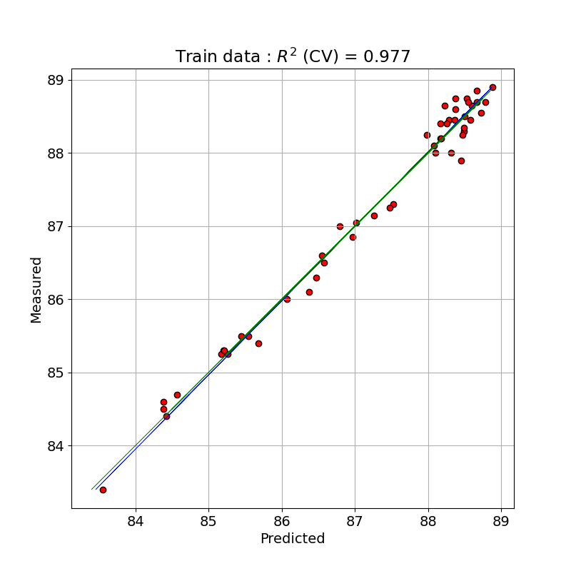
for Training data
R2 calib: 0.985
R2 CV: 0.977
MSE calib: 0.035
MSE CV: 0.052
トレーニングデータで PLS のモデルで予測(クロスバリデーションと比較)した値と測定値とを単回帰したプロットを示しました。クロスバリデーションをした予測で決定係数が 0.977 となっており、よくフィッティングできています。
# Plot regression and figures of merit
rangey = max(y_train) - min(y_train)
rangex = max(y_train_c) - min(y_train_c)

# Fit a line to the CV vs response
z = np.polyfit(y_train, y_train_c, 1)
fig, ax = plt.subplots(figsize=(8, 8))

# Plot the best fit line
ax.plot(np.polyval(z, y_train), y_train, c='blue', linewidth=0.5)

# Plot the ideal 1:1 line
ax.plot(y_train, y_train, color='green', linewidth=0.5)

ax.scatter(y_train_c, y_train, c='red', edgecolors='k')
plt.title('Train data : $R^{2}$ (CV) = ' + '{:.3f}'.format(score_train_cv))
plt.xlabel('Predicted')
plt.ylabel('Measured')
ax.axis('equal')
plt.grid()

plt.savefig('octane_003.png')
plt.show()
テストデータで予測
最適とした PLS 回帰モデルをテストデータに適用して、予測パフォーマンスを確認します。
# Fit to the entire dataset
pls_opt.fit(X_test, y_test)
y_pred = pls_opt.predict(X_test)

# Calculate scores for calibration and cross-validation
score_pred = r2_score(y_test, y_pred)

# Calculate mean squared error for calibration and cross validation
mse_pred = mean_squared_error(y_test, y_pred)

print('for Test data')
print('R2 pred: %5.3f' % score_pred)
print('MSE pred: %5.3f' % mse_pred)
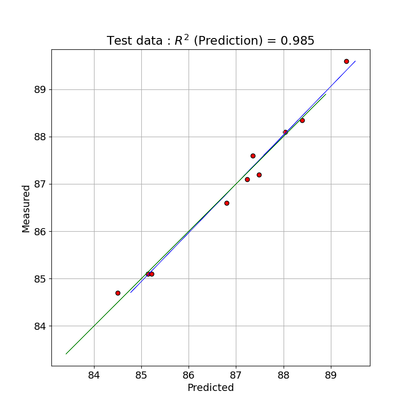
for Test data
R2 pred: 0.985
MSE pred: 0.033
幸い、テストデータでも良いフィッテイングが得られました。
テストデータで PLS のモデルで予測した値と測定値とを単回帰したプロットを示しました。
# Plot regression and figures of merit
rangey = max(y_test) - min(y_test)
rangex = max(y_pred) - min(y_pred)

# Fit a line to the CV vs response
z = np.polyfit(y_test, y_pred, 1)
fig, ax = plt.subplots(figsize=(8, 8))

# Plot the best fit line
ax.plot(np.polyval(z, y_test), y_test, c='blue', linewidth=0.5)

# Plot the ideal 1:1 line
ax.plot(y_train, y_train, color='green', linewidth=0.5)

ax.scatter(y_pred, y_test, c='red', edgecolors='k')
plt.title('Test data : $R^{2}$ (Prediction) = ' + '{:.3f}'.format(score_pred))
plt.xlabel('Predicted')
plt.ylabel('Measured')
ax.axis('equal')
plt.grid()

plt.savefig('octane_004.png')
plt.show()
PLS 回帰における変数選択の改善方法が参考サイト [3] にありますので、今後、確認してみたいと思います。
※ テストデータの評価に間違いがありましたので修正しました。[2023-07-07]
参考サイト
- bitWalk's: 【備忘録】Rのplsパッケージの使い方 [2017-06-18]
- Partial Least Squares Regression in Python [2018-06-14]
- A variable selection method for PLS in Python [2018-07-04]
にほんブログ村

#オープンソース